On the importance of interpretable code - Transformers

The following chapter serves as a clean, first principles introduction to Transformers. In this chapter, we will implement GPT-2 (Radford et al., 2018) in PyTorch. The architectural choices closely follow those used by the TransformerLens library (Nanda and Bloom, 2022), which we will heavily make use of in upcoming sections.

The exercises, taken from Arena 3.0, are written to accompany Neel Nanda’s TransformerLens for doing mechanistic interpretability research on GPT-2 style language models.

Outline of the chapter

The rest of the blogpost is organised as follows:

• Section 2.1 will be dedicated to an in depth introduction to the Transformer. We will go through the paper in an annotated fashion, accompanying the explanation with a line-by-line implementation.
• Section 2.2 will introduce us to transformers—what their function is, how information moves inside a transformer and what inputs and outputs they take.
• Section 2.3, where we will implement a transformer from scratch, using only PyTorch tensor operations. This will give us a good understanding of how transformers work, and how to use them. We do this by going module-by-module, as to appreciate every building block of this amazing architecture.
• Section 2.4, instead, we will teach us how to train our transformer from scratch.
• In Section 2.5, finally, we will learn how to sample from a transformer. This will involve implementing a few different sampling methods, and writing a caching system which can reuse computations from previous forward passes to improve model’s text generation efficiency.

2.1 The Transformer

The Transformer is a groundbreaking architecture that revolutionized the field of natural language processing. It introduced a new approach to sequence-to-sequence modeling, focusing on attention mechanisms to process data in parallel, rather than relying on recurrent connections. When first introduced, it was able to outperform the state of the art in machine translation, and set a new benchmark for the field.

I think people underestimate or better, have to take for granted this work. It is the foundation of all the success we see in the field of NLP today. It is the work that allows us to build models like GPT-4, that can generate human-like text, that can answer questions, that can write code, that can do all sorts of things. It is a masterpiece of simplicity and elegance.

Truly, the Transformer is a stunning architecture.

2.2 The explained Transformer

The goal of reducing sequential computation was already well documented in different projects that were being developed co-occurrently with the Transformer. Works such as the Extended Neural GPU by Kaiser and Sutskever (2016), ByteNet by Kalchbrenner et al. (2017) and ConvS2S by Gehring et al. (2017), aimed at using CNNs as basic building blocks to compute hidden representations in parallel for all input and output positions. In these models, the number of operations required to relate signals from two arbitrary input or output positions, grows in the distance between the positions: linearly for ConvS2S and logarithmically for ByteNet. This makes it cumbersome to learn distant dependencies. In the Transformer, this is reduced to a constant number of operations, albeit at the cost of reduced effective resolution, due to averaging attention-weighted positions, an effect tamed by Multi-Head Attention.

But what is effective resolution? In the context of neural networks and specifically when discussing models like the Transformer, it refers to the model’s ability to distinguish and process fine-grained details within the data it works with. The Transformer model uses attention mechanisms to weigh and prioritize different parts of the input data. The process of averaging attention-weighted positions to calculate the output can lead to a reduction in the effective resolution because it may blend together distinct elements of the input into a more uniform representation. This blending can make it harder for the model to pick out and utilize specific, fine-grained details in later processing stages. However, the Transformer addresses this challenge through Multi-Head Attention, which allows it to maintain a higher effective resolution by concurrently processing the data in multiple ways, thereby capturing a wider array of details and nuances.

Self-attention is an attention mechanism relating different positions of a single sequence in order to compute a representation of the sequence. Self-attention has been used successfully in a variety of tasks, however, the Transformer was the first transduction model relying entirely on self-attention to compute representations of its input and output without using sequence aligned RNNs or convolution.

Model Architecture

Most competitive neural sequence models have an encoder-decoder structure (Bahdanau et al., 2016). Here, the encoder maps an input sequence of symbol representations $\left(x_1, \dots, x_n\right)$ to a sequence of continuous representations $\boldsymbol{z} =\left(z_1, \dots, x_n\right)$. Given $\boldsymbol{z}$, the decoder then generates an output sequence $\left(y_1, \dots, y_m\right)$ of symbols one element at a time. At each step, the mode is said to be autoregressive (Graves, 2014), “consuming” the previously generated symbols as additional input when generating the text.

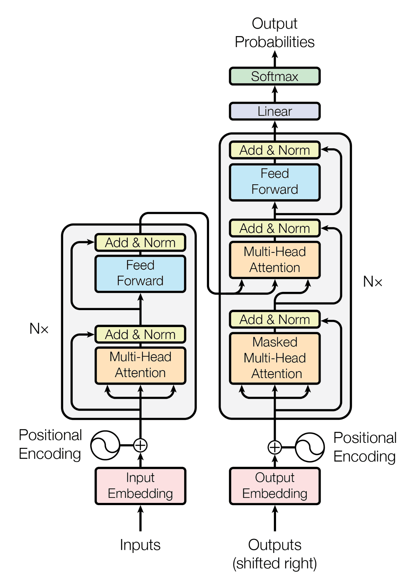
Encoder and Decoder stacks

Encoder

The encoder is composed of a stack of $N = 6$ identical layers.

def clones(module, N):
    "Produce N identical layers."
    return nn.ModuleList([copy.deepcopy(module) for _ in range(N)])

class Encoder(nn.Module):
    "Core encoder is a stack of N layers"
 
    def __init__(self, layer, N):
        super(Encoder, self).__init__()
        self.layers = clones(layer, N)
        self.norm = nn.LayerNorm(layer.size)
 
    def forward(self, x, mask):
        "Pass the input (and mask) through each layer in turn"
        for layer in self.layers:
            x = layer(x, mask)
        return self.norm(x)

We employ a residual connection (He et al., 2015) around each of the two sub-layers, followed by layer normalization. That is, the output of each sub-layer is LayerNorm(x + SubLayer(x)), where SubLayer(x) is the function implemented by the sub-layer itself. We also apply dropout to the output of each sub-layer, before it is added to the sub-layer input and normalized.

To facilitate the residual connections, all sub-layers in the models, as well as the embedding layers, produce outputs of dimension $d_{model} = 512$.

class SublayerConnection(nn.Module):
    """
    A residual connection followed by a layer norm.
    Note for code simplicity the norm is first as opposed to last
    """
 
    def __init__(self, size, dropout):
        super(SublayerConnection, self).__init__()
        self.norm = nn.LayerNorm(size)
        self.dropout = nn.Dropout(dropout)
 
    def forward(self, x, mask):
        "Apply residual connection to any sublayer with the same size"
        return x + self.dropout(sublayer(self.norm(x)))

Each layer has two sub-layers. The first is a multi-head self-attention mechanism, and the second is a simple, position-wise fully connected feed-forward neural network.

class EncoderLayer(nn.Module):
    "Encoder is made up of self-attn and ffnn (defined below)"
 
    def __init__(self, size, self_attn, ffnn, dropout):
        super(EncoderLayer, self).__init__()
        self.size = size
        self.self_attn = self.attn
        self.ffnn = ffnn
        self.sublayer = clones(SublayerConnection(size, dropout), 2)
 
    def forward(self, x, mask):
        "Figure above, coded."
        x = self.sublayer[0](x, lambda x: self.self_attn(x, x, x, mask))
        return self.sublayer[1](x, self.ffnn)

Decoder

Similarly, the decoder is also composed of a stack of $N = 6$ identical layers.

class Decoder(nn.Module):
    "Core Decoder is a stack of N layers with masking."
 
    def __init__(self, layer, N):
        super(Decoder, self).__init__()
        self.layers = clones(layer, N)
        self.norm = nn.LayerNorm(layer.size)
 
    def forward(self, x, mask):
        "Pass the input (and mask) through each layer in turn"
        for layer in self.layers:
            x = layer(x, memory, src_mask, tgt_mask)
        return self.norm(x)

In addition to the two sub-layers in each encoder layer, the decoder inserts a third sub-layer, which performs multi-head attention over the output of the encoder stack. Similar to the encoder, we employ residual connections around each of the sub-layers, followed by layer normalization.

class DecoderLayer(nn.Module):
    "Decoder is made of self-attn, src-attn, and feed forward (defined below)"
 
    def __init__(self, size, self_attn, src_attn, feed_forward, dropout):
        super(DecoderLayer, self).__init__()
        self.size = size
        self.self_attn = self_attn
        self.src_attn = src_attn
        self.feed_forward = feed_forward
        self.sublayer = clones(SublayerConnection(size, dropout), 3)
 
    def forward(self, x, memory, src_mask, tgt_mask):
        "Follow Figure 1 (right) for connections."
        m = memory
        x = self.sublayer[0](x, lambda x: self.self_attn(x, x, x, tgt_mask))
        x = self.sublayer[1](x, lambda x: self.src_attn(x, m, m, src_mask))
        return self.sublayer[2](x, self.feed_forward)

We also modify the self-attention sub-layer in the decoder stack to prevent positions from attending to subsequent ones. This masking, combined with the fact that the output embeddings are offset by one position, ensures that the predictions for position $i$ can depend only on the known outputs at positions $j<i$.

def subsequent_mask(size):
	"Mask out subsequent positions."
	attn_shape = (1, size, size)
	subsequent_mask = torch.triu(torch.ones(attn_shape), diagonal=1).type(torch.uint8)
	return subsequent_mask == 0

2.3 Implementing a Transformer from scratch

This section details a ground-up implementation of a GPT-2 style Transformer, using only PyTorch tensor operations. We’re eschewing pre-built Transformer modules to gain a deep, intuitive understanding of each component. This is not merely an academic exercise; a firm grasp of the fundamentals is crucial for effective interpretability research. By building the model piece by piece, we can appreciate the role of each element and how they interact. We’ll be adhering closely to the architecture used in the TransformerLens library, providing a solid foundation for later work.

We proceed module-by-module, starting with the foundational components: embeddings and positional encoding.

Embeddings and Positional Encoding: Representing Tokens and Their Positions

The first step in processing text with a Transformer is to convert the raw tokens (words or sub-word units) into numerical representations that the model can operate on. This is achieved through embeddings.

An embedding is a vector in a high-dimensional space (typically hundreds of dimensions). Each unique token in the vocabulary is assigned a unique embedding vector. Crucially, semantically similar tokens tend to have embeddings that are closer together in this space, allowing the model to capture relationships between words.

import torch
import torch.nn as nn
import math
from einops import rearrange, reduce, repeat
 
"""
Dimension key for tensor shape suffixes (Noam Shazeer you are a legend):
 
B: batch size
L: sequence length (input sequence)
M: memory length (sequence being attended to)
D: model dimension (d_model/embedding dimension)
V: vocabulary size
F: feed-forward hidden dimension
H: number of attention heads
K: size of each attention head (d_k = D/H)
 
Example: hidden_BLD represents a tensor with shape (batch_size, seq_len, d_model)
"""
 
class TokenEmbedding(nn.Module):
    """Token embedding layer that maps token IDs to dense vectors.
    
    The embedding vectors are scaled by sqrt(d_model) to prevent dot products in 
    attention from growing too large, which can lead to extremely small gradients.
    
    Args:
        d_model (int): Model dimension D
        vocab_size (int): Vocabulary size V
    """
    def __init__(self, d_model: int, vocab_size: int):
        super().__init__()
        self.embedding_VD = nn.Embedding(vocab_size, d_model)
        self.d_model = d_model
 
    def forward(self, token_id_BL: torch.Tensor) -> torch.Tensor:
        """Map token IDs to scaled embedding vectors.
        
        Args:
            token_id_BL: Input token IDs of shape (B, L)
            
        Returns:
            embed_BLD: Token embeddings of shape (B, L, D)
        """
        embed_BLD = self.embedding_VD(token_id_BL) * math.sqrt(self.d_model)
        return embed_BLD

The nn.Embedding layer acts as a lookup table. Given a token index, it returns the corresponding embedding vector. The multiplication by math.sqrt(self.d_model) is a critical detail from the “Attention is All You Need” paper. It scales the embeddings to prevent the dot products in the subsequent attention mechanism from becoming excessively large, which can lead to instability during training (vanishing gradients).

Transformers, unlike recurrent neural networks (RNNs), do not inherently process sequential information in order. They are permutation-invariant; the order of the input tokens doesn’t intrinsically affect the output. To address this, we need to explicitly encode the position of each token within the sequence. This is the role of Positional Encoding.

The original Transformer paper utilizes a sinusoidal positional encoding scheme:

class PositionalEncoding(nn.Module):
    """Adds positional information to token embeddings using sinusoidal encodings.
    
    Uses a combination of sine and cosine functions with geometrically increasing wavelengths
    to create unique position-dependent patterns. These patterns allow the model to learn
    relative positions between tokens.
    
    Args:
        d_model (int): Model dimension D
        max_len (int): Maximum sequence length supported
    """
    def __init__(self, d_model: int, max_len: int = 5000):
        super().__init__()
        self.d_model = d_model
        
        # Create position encodings
        pos_L = torch.arange(0, max_len, dtype=torch.float).unsqueeze(1)
        div_term = torch.exp(torch.arange(0, d_model, 2).float() * (-math.log(10000.0) / d_model))
        
        # Initialize positional encoding buffer
        pe_LD = torch.zeros(max_len, d_model)
        pe_LD[:, 0::2] = torch.sin(pos_L * div_term)
        pe_LD[:, 1::2] = torch.cos(pos_L * div_term)
        pe_1LD = pe_LD.unsqueeze(0)  # Add batch dimension
        
        # Register buffer (not a parameter, but should be saved with model)
        self.register_buffer('pe_1LD', pe_1LD)
 
    def forward(self, hidden_BLD: torch.Tensor) -> torch.Tensor:
        """Add positional encodings to token embeddings.
        
        Args:
            hidden_BLD: Token embeddings of shape (B, L, D)
            
        Returns:
            pos_hidden_BLD: Position-aware embeddings of shape (B, L, D)
        """
        pos_hidden_BLD = hidden_BLD + self.pe_1LD[:, :hidden_BLD.size(1)]
        return pos_hidden_BLD

This code generates a matrix pe where each row represents the positional encoding for a specific position in the sequence. The encoding is created using sine and cosine functions with varying frequencies. The div_term controls these frequencies, ensuring a mix of high-frequency (for distinguishing nearby positions) and low-frequency (for capturing long-range dependencies) components. This creates a unique, position-dependent “signature” that is added to the token embeddings.

The use of register_buffer ensures that the positional encoding matrix pe is saved and loaded along with the model’s state, even though it’s not a trainable parameter.

Importantly, the positional encoding is added to the token embeddings. This allows the model to learn to jointly attend to both the semantic content of the token (from the embedding) and its position in the sequence (from the positional encoding).

With embeddings and positional encodings in place, we are now prepared to delve into the core of the Transformer: the attention mechanism.

2.3.2 Attention: The Heart of the Transformer

Attention is the mechanism that allows the Transformer to weigh the importance of different parts of the input sequence when processing each token. It’s what enables the model to capture long-range dependencies and contextual relationships so effectively. We’ll start with the scaled dot-product attention, the fundamental building block, and then build up to multi-head attention.

Scaled Dot-Product Attention

Scaled dot-product attention takes three inputs: queries (Q), keys (K), and values (V). These are all linear transformations of the input embeddings (or the output of a previous layer). Think of them as different “views” of the same underlying information.

1. Dot Product and Scaling: We compute the dot product of the queries with all keys. The dot product measures the similarity between a query and each key. We then scale these dot products by dividing by the square root of the key dimension (d_k). This scaling is crucial to prevent the dot products from becoming too large, which can lead to extremely small gradients during backpropagation (the vanishing gradient problem again!).

2. Softmax: A softmax function is applied to the scaled dot products. This converts the similarity scores into probabilities, representing the attention weights. These weights determine how much each value contributes to the final output.

3. Weighted Sum: Finally, we compute a weighted sum of the values, using the attention weights. This produces the output of the attention mechanism, which is a context-aware representation of the input.

def scaled_dot_product_attention(
    query_BHLK: torch.Tensor,
    key_BHMK: torch.Tensor,
    value_BHMK: torch.Tensor,
    mask_1LM: torch.Tensor = None
) -> tuple[torch.Tensor, torch.Tensor]:
    """Compute scaled dot-product attention.
    
    Calculates attention scores between queries and keys, then uses these scores
    to create a weighted sum of values. The dot products are scaled by 1/sqrt(K)
    to counteract growth in variance with increasing key dimension.
    
    Args:
        query_BHLK: Query tensor of shape (B, H, L, K)
        key_BHMK: Key tensor of shape (B, H, M, K)
        value_BHMK: Value tensor of shape (B, H, M, K)
        mask_1LM: Optional mask tensor of shape (1, L, M) or (1, 1, M)
        
    Returns:
        output_BHLK: Weighted combination of values (B, H, L, K)
        attn_BHLM: Attention weights (B, H, L, M)
    """
    # Compute attention scores
    scores_BHLM = torch.einsum('bhlk,bhmk->bhlm', [query_BHLK, key_BHMK]) / math.sqrt(query_BHLK.size(-1))
    
    # Apply mask if provided
    if mask_1LM is not None:
        scores_BHLM = scores_BHLM.masked_fill(mask_1LM == 0, -1e9)
    
    # Compute attention weights and weighted sum
    attn_BHLM = torch.softmax(scores_BHLM, dim=-1)
    output_BHLK = torch.einsum('bhlm,bhmk->bhlk', [attn_BHLM, value_BHMK])
    
    return output_BHLK, attn_BHLM

The mask argument is crucial for two reasons:

• Padding: Input sequences often have varying lengths. We pad shorter sequences to a uniform length. The mask prevents the model from attending to these padding tokens.
• Causal Attention (for Decoders): In a decoder (like in GPT-2), we don’t want the model to “peek” at future tokens when generating text. The mask prevents a token from attending to tokens that occur later in the sequence. This is causal or masked self-attention.

The shapes of the tensors are important to understand. We’ll see batch, heads (for multi-head attention, explained next), seq_len, and d_k or d_v (the dimensions of the keys/queries and values, respectively).

Multi-Head Attention

Multi-head attention enhances the basic scaled dot-product attention by allowing the model to attend to different aspects of the input simultaneously. Instead of performing a single attention calculation, we perform multiple attention calculations in parallel, each with different learned linear projections of the queries, keys, and values.

Think of it like having multiple “experts,” each focusing on a different aspect of the input. One head might focus on grammatical relationships, another on semantic similarity, and another on long-range dependencies.

class MultiHeadAttention(nn.Module):
    """Multi-head attention mechanism that allows the model to jointly attend to information 
    from different representation subspaces at different positions.
    
    Each head performs scaled dot-product attention on a lower-dimensional projection
    of the input, allowing the model to capture different types of dependencies between
    tokens.
    
    Args:
        d_model (int): Model dimension D
        num_heads (int): Number of attention heads H
    """
    def __init__(self, d_model: int, num_heads: int):
        super().__init__()
        assert d_model % num_heads == 0, "d_model must be divisible by num_heads"
 
        self.d_model = d_model
        self.num_heads = num_heads
        self.head_dim = d_model // num_heads
 
        # Linear projections
        self.W_q_DHD = nn.Linear(d_model, d_model)
        self.W_k_DHD = nn.Linear(d_model, d_model)
        self.W_v_DHD = nn.Linear(d_model, d_model)
        self.W_o_DHD = nn.Linear(d_model, d_model)
 
    def forward(
        self,
        query_BLD: torch.Tensor,
        key_BMD: torch.Tensor,
        value_BMD: torch.Tensor,
        mask_1LM: torch.Tensor = None
    ) -> torch.Tensor:
        """Compute multi-head attention.
        
        Projects inputs into multiple heads, applies scaled dot-product attention
        independently to each head, and combines results.
        
        Args:
            query_BLD: Query tensor of shape (B, L, D)
            key_BMD: Key tensor of shape (B, M, D)
            value_BMD: Value tensor of shape (B, M, D)
            mask_1LM: Optional mask tensor of shape (1, L, M) or (1, 1, M)
            
        Returns:
            output_BLD: Attention output of shape (B, L, D)
        """
        # Linear projections and split into heads
        query_BHLK = rearrange(self.W_q_DHD(query_BLD), 'b l (h k) -> b h l k', h=self.num_heads)
        key_BHMK = rearrange(self.W_k_DHD(key_BMD), 'b m (h k) -> b h m k', h=self.num_heads)
        value_BHMK = rearrange(self.W_v_DHD(value_BMD), 'b m (h k) -> b h m k', h=self.num_heads)
 
        # Apply scaled dot-product attention
        attn_out_BHLK, _ = scaled_dot_product_attention(query_BHLK, key_BHMK, value_BHMK, mask_1LM)
        
        # Combine heads and project
        output_BLD = self.W_o_DHD(rearrange(attn_out_BHLK, 'b h l k -> b l (h k)'))
        
        return output_BLD

The key steps are:

1. Linear Projections: We use nn.Linear layers (W_q, W_k, W_v) to project the queries, keys, and values into different subspaces. These projections are learned during training.

2. Splitting into Heads: We reshape and transpose the projected Q, K, and V tensors to create multiple “heads.” This is done using .view() and .transpose().

3. Scaled Dot-Product Attention: We apply scaled_dot_product_attention to each head independently.

4. Concatenation and Final Projection: The outputs from all heads are concatenated and then passed through a final linear layer (W_o). This combines the information from all the heads into a single output vector.

The contiguous() call ensures that the tensor is stored in a contiguous block of memory, which can improve performance.

2.3.3 Position-wise Feed-Forward Networks

After the attention mechanism, each Transformer layer includes a position-wise feed-forward network (FFN). This is a simple, fully connected network that is applied to each position in the sequence independently. It provides additional non-linearity and allows the model to learn more complex representations.

class PositionwiseFeedForward(nn.Module):
    """Position-wise feed-forward network applied independently to each position.
    
    Consists of two linear transformations with a ReLU/GELU activation in between.
    The inner dimension is typically larger than the model dimension, allowing the
    network to learn more complex functions.
    
    Args:
        d_model (int): Model dimension D
        d_ff (int): Feed-forward inner dimension F
    """
    def __init__(self, d_model: int, d_ff: int):
        super().__init__()
        self.W1_DF = nn.Linear(d_model, d_ff)
        self.W2_FD = nn.Linear(d_ff, d_model)
        self.gelu = nn.GELU()  # GPT-2 uses GELU activation
 
    def forward(self, hidden_BLD: torch.Tensor) -> torch.Tensor:
        """Apply position-wise feed-forward transformation.
        
        Args:
            hidden_BLD: Input tensor of shape (B, L, D)
            
        Returns:
            output_BLD: Transformed tensor of shape (B, L, D)
        """
        # Project up to higher dimension
        hidden_BLF = self.gelu(self.W1_DF(hidden_BLD))
        
        # Project back to model dimension
        output_BLD = self.W2_FD(hidden_BLF)
        
        return output_BLD

The FFN typically consists of two linear layers with a non-linear activation function (ReLU or GELU) in between. The inner dimension (d_ff) is usually larger than the model dimension (d_model). This “expansion” and “contraction” of the representation allows the model to learn more complex features.

2.3.4 Layer Normalization and Residual Connections

Two more crucial components are layer normalization and residual connections. These are essential for stable training and allowing the model to learn deeper representations.

Layer Normalization

Layer normalization (LayerNorm) normalizes the activations of each layer across the feature dimension. This helps to stabilize training and prevent the activations from becoming too large or too small. It’s similar in spirit to batch normalization, but it operates on a per-example basis, making it suitable for sequence models.

class LayerNorm(nn.Module):
    """Layer normalization module that normalizes inputs across the feature dimension.
    
    Computes mean and standard deviation across the feature dimension (D) for each
    position in each sequence in the batch, then normalizes the inputs using these
    statistics. Learned scale (gamma) and shift (beta) parameters are applied after
    normalization.
    
    Args:
        d_model (int): Model dimension D
        eps (float): Small constant for numerical stability
    """
    def __init__(self, d_model: int, eps: float = 1e-6):
        super().__init__()
        self.gamma_D = nn.Parameter(torch.ones(d_model))
        self.beta_D = nn.Parameter(torch.zeros(d_model))
        self.eps = eps
 
    def forward(self, hidden_BLD: torch.Tensor) -> torch.Tensor:
        """Apply layer normalization.
        
        Args:
            hidden_BLD: Input tensor of shape (B, L, D)
            
        Returns:
            norm_BLD: Normalized tensor of shape (B, L, D)
        """
        # Compute statistics across feature dimension
        mean_BL1 = hidden_BLD.mean(dim=-1, keepdim=True)
        std_BL1 = hidden_BLD.std(dim=-1, keepdim=True)
        
        # Normalize and apply learned parameters
        norm_BLD = self.gamma_D * (hidden_BLD - mean_BL1) / (std_BL1 + self.eps) + self.beta_D
        return norm_BLD

LayerNorm computes the mean and standard deviation across the last dimension (the feature dimension, d_model). It then normalizes the input using these statistics and applies learned scale (gamma) and shift (beta) parameters. The small constant eps is added for numerical stability.

Residual Connections

Residual connections (or skip connections) add the input of a sub-layer (like the attention layer or the FFN) to its output. This creates a “shortcut” path for the gradient during backpropagation, which helps to mitigate the vanishing gradient problem and allows for training much deeper networks.

class ResidualConnection(nn.Module):
  def __init__(self, size: int, dropout: float):
        super(ResidualConnection, self).__init__()
        self.norm = LayerNorm(size)
        self.dropout = nn.Dropout(dropout)
 
  def forward(self, x: torch.Tensor, sublayer: Callable) -> torch.Tensor:
        """Applies a residual connection to any sublayer with the same size."""
        return x + self.dropout(sublayer(self.norm(x)))

The ResidualConnection module combines layer normalization, the sublayer (e.g., attention or FFN), dropout, and the residual connection. We first normalize the input using LayerNorm, then apply the sublayer, then apply dropout (for regularization), and finally add the original input to the output.

2.3.5 Putting It All Together: The Transformer Block

Now we can combine all these components into a single Transformer block. This is the fundamental building block of both the encoder and decoder in the original Transformer, and of the decoder-only GPT-2 model.

from typing import Callable
 
class TransformerBlock(nn.Module):
    def __init__(self, d_model: int, num_heads: int, d_ff: int, dropout: float):
        super().__init__()
        self.attention = MultiHeadAttention(d_model, num_heads)
        self.feed_forward = PositionwiseFeedForward(d_model, d_ff)
        self.residual1 = ResidualConnection(d_model, dropout)
        self.residual2 = ResidualConnection(d_model, dropout)
 
    def forward(self, x: torch.Tensor, mask: torch.Tensor) -> torch.Tensor:
        """
        x: (batch, seq_len, d_model)
        mask: (batch, 1, seq_len) or (batch, 1, 1, seq_len)
        Returns: (batch, seq_len, d_model)
        """
        x = self.residual1(x, lambda x: self.attention(x, x, x, mask))
        x = self.residual2(x, self.feed_forward)
        return x

The TransformerBlock consists of:

1. Multi-Head Attention: The input x is passed through the multi-head attention mechanism (with itself as query, key, and value, for self-attention).
2. Residual Connection and LayerNorm (1): The output of the attention layer is added to the original input x (residual connection), and layer normalization is applied.
3. Position-wise Feed-Forward Network: The output is then passed through the FFN.
4. Residual Connection and LayerNorm (2): Another residual connection and layer normalization are applied.

This block is repeated multiple times (e.g., 12 times in GPT-2 small) to create a deep Transformer model.

2.3.6 The Full GPT-2 Model

Finally, we can assemble the complete GPT-2 model. This involves stacking multiple TransformerBlocks, along with the initial token and positional embeddings, and a final linear layer to project the output to the vocabulary size.

class GPT2(nn.Module):
    def __init__(self, vocab_size: int, d_model: int, num_heads: int, d_ff: int, num_layers: int, dropout: float, max_len: int = 1024):
        super().__init__()
        self.token_embedding = TokenEmbedding(d_model, vocab_size)
        self.positional_encoding = PositionalEncoding(d_model, max_len)
        self.transformer_blocks = nn.ModuleList(
            [TransformerBlock(d_model, num_heads, d_ff, dropout) for _ in range(num_layers)]
        )
        self.dropout = nn.Dropout(dropout)
        self.final_ln = LayerNorm(d_model)
        self.lm_head = nn.Linear(d_model, vocab_size) # Language modeling head
 
    def forward(self, x: torch.Tensor, mask: torch.Tensor = None) -> torch.Tensor:
        """
        x: (batch, seq_len) - Input sequence of token indices.
        mask: (batch, 1, seq_len) or (batch, 1, 1, seq_len)
 
        Returns:
            logits: (batch, seq_len, vocab_size) - Logits for next-token prediction.
        """
        x = self.token_embedding(x)
        x = self.positional_encoding(x)
        x = self.dropout(x)
 
        if mask is None:
            # Create causal mask using einops
            seq_len = x.size(1)
            mask = repeat(torch.tril(torch.ones(seq_len, seq_len)), 'i j -> b 1 i j', b=1)
            mask = mask.to(x.device)
 
        for block in self.transformer_blocks:
            x = block(x, mask)
 
        x = self.final_ln(x)
        logits = self.lm_head(x)
        return logits

The GPT2 model combines all the components we’ve built:

1. Token and Positional Embeddings: The input token indices are converted to embeddings, and positional encodings are added.
2. Transformer Blocks: The combined embeddings are passed through a stack of TransformerBlocks.
3. Causal Mask: If no mask is provided, it creates a causal mask.
4. Final Layer Normalization: Layer normalization is applied to the output of the final Transformer block.
5. Language Modeling Head: A final linear layer (lm_head) projects the output to the vocabulary size, producing logits. These logits can be converted to probabilities using a softmax function to predict the next token in the sequence.

2.4 Training the Transformer

This section outlines the training process for the GPT-2 style Transformer we implemented in Section 2.3. We’ll cover the loss function, optimization, and key considerations for training such a large language model.

2.4.1 Loss Function: Cross-Entropy Loss

The standard loss function for training language models is the cross-entropy loss. GPT-2, being an autoregressive language model, is trained to predict the next token in a sequence given the preceding tokens. Cross-entropy loss measures the difference between the predicted probability distribution over the vocabulary and the actual (one-hot encoded) next token.

import torch
import torch.nn.functional as F
 
def cross_entropy_loss(logits_BLV: torch.Tensor, target_token_ids_BL: torch.Tensor) -> torch.Tensor:
    """
    Calculates the cross-entropy loss.
 
    Args:
        logits_BLV: (batch, seq_len, vocab_size) - Logits for next-token prediction.
        target_token_ids_BL: (batch, seq_len) - Indices of the correct next tokens.
 
    Returns:
        loss: (1) - The mean cross-entropy loss over the batch and sequence length.
    """
    # Flatten logits and targets to (B*L, V) and (B*L) for F.cross_entropy
    log_probs_BLV = F.log_softmax(logits_BLV, dim=-1)
    loss = F.cross_entropy(logits_BLV.view(-1, logits_BLV.size(-1)), target_token_ids_BL.view(-1))
    return loss

We use F.cross_entropy, which efficiently combines the log-softmax and negative log-likelihood (NLL) loss calculations. We reshape the logits_BLV and target_token_ids_BL tensors to be compatible with F.cross_entropy. The loss is averaged over both the batch and sequence length dimensions. Note the use of Shazeerian variable names.

2.4.2 Optimizer: AdamW

The AdamW optimizer is a variant of Adam that incorporates weight decay directly into the optimization step, rather than adding it as an L2 regularization term to the loss. This has been shown to be more effective for training Transformers. A lot of discourse has been had around optimizers as of late, with second order methods like Shampoo and Muon being thrown around. I find this to be an interesting area of research, but also a massive rabbit hole. Optimizers are a bit of a black art, and the reason papers alone can’t provide strong evidence is because if they contain a mistake (like an untuned hyperparameter), nothing ever happens.

def configure_optimizers(model: nn.Module, learning_rate: float, weight_decay: float, betas: tuple[float, float] = (0.9, 0.999)):
    """
    Configures the AdamW optimizer.  Separates parameters for weight decay.
 
    Args:
        model: The PyTorch model to optimize.
        learning_rate: The learning rate.
        weight_decay: The weight decay coefficient.
        betas: The beta parameters for AdamW.
 
    Returns:
        optimizer: The configured AdamW optimizer.
    """
 
    # Separate parameters for weight decay (typically biases and LayerNorm parameters are excluded)
    param_dict = {pn: p for pn, p in model.named_parameters()}
    param_dict = {pn: p for pn, p in param_dict.items() if p.requires_grad}
    decay_params = [p for n, p in param_dict.items() if p.dim() >= 2]
    nodecay_params = [p for n, p in param_dict.items() if p.dim() < 2]
    optim_groups = [
        {'params': decay_params, 'weight_decay': weight_decay},
        {'params': nodecay_params, 'weight_decay': 0.0}
    ]
    num_decay_params = sum(p.numel() for p in decay_params)
    num_nodecay_params = sum(p.numel() for p in nodecay_params)
    print(f"num decayed parameter tensors: {len(decay_params)}, with {num_decay_params:,} parameters")
    print(f"num non-decayed parameter tensors: {len(nodecay_params)}, with {num_nodecay_params:,} parameters")
    # Create AdamW optimizer
    optimizer = torch.optim.AdamW(optim_groups, lr=learning_rate, betas=betas)
    return optimizer
 

The configure_optimizers function separates the model’s parameters into two groups: those that will be subject to weight decay (typically weights in linear layers and embeddings) and those that won’t (typically biases and LayerNorm parameters). This is a common practice in Transformer training. We then create an AdamW optimizer with different weight decay settings for these two groups.

2.4.3 Training Loop

The training loop iterates over the training data, computes the loss, and updates the model’s parameters.

def train(model: nn.Module, optimizer: torch.optim.Optimizer, train_data: torch.utils.data.DataLoader, num_epochs: int, device: str = 'cuda'):
    """
    Trains the GPT-2 model.
 
    Args:
        model: The GPT-2 model.
        optimizer: The optimizer.
        train_data: DataLoader for the training data.
        num_epochs: Number of training epochs.
        device: Device to train on ('cuda' or 'cpu').
    """
    model.to(device)
    model.train()
 
    for epoch in range(num_epochs):
        for batch_idx, (input_ids_BL, target_ids_BL) in enumerate(train_data):
            input_ids_BL = input_ids_BL.to(device)
            target_ids_BL = target_ids_BL.to(device)
 
            # Forward pass
            logits_BLV = model(input_ids_BL)
 
            # Calculate loss
            loss = cross_entropy_loss(logits_BLV, target_ids_BL)
 
            # Backward pass and optimization
            optimizer.zero_grad()
            loss.backward()
            optimizer.step()
 
            if batch_idx % 100 == 0:
                print(f'Epoch: {epoch+1}/{num_epochs}, Batch: {batch_idx+1}/{len(train_data)}, Loss: {loss.item():.4f}')

This train function encapsulates the core training process:

1. Data Loading: We iterate through batches of data from the train_data DataLoader.
2. Forward Pass: The input sequence (input_ids_BL) is passed through the model to obtain the logits (logits_BLV).
3. Loss Calculation: The cross-entropy loss is computed between the logits and the target tokens (target_ids_BL).
4. Backward Pass: The gradients of the loss with respect to the model’s parameters are calculated.
5. Optimization Step: The optimizer updates the model’s parameters based on the computed gradients.
6. Logging: The loss is printed periodically to monitor training progress.

2.4.4 Key Training Considerations

• Data Preprocessing: High-quality data and appropriate tokenization are essential. GPT-2 uses byte-pair encoding (BPE).
• Learning Rate Schedule: A learning rate scheduler (e.g., cosine annealing or a linear warmup followed by decay) is crucial for optimal convergence.
• Gradient Clipping: Clipping the gradients to a maximum norm can prevent exploding gradients, especially during the early stages of training.
• Mixed Precision Training: Using mixed precision (e.g., FP16) can significantly speed up training and reduce memory usage on GPUs that support it. PyTorch’s torch.cuda.amp provides tools for this.
• Batch Size: Larger batch sizes generally lead to more stable training, but are limited by GPU memory.
• Sequence Length: The maximum sequence length is a key hyperparameter. Longer sequences allow the model to capture longer-range dependencies, but increase computational cost.
• Regularization: Dropout is used within the Transformer blocks. Weight decay (as part of AdamW) also acts as a regularizer.
• Distributed Training: For very large models, distributed training across multiple GPUs or machines is often necessary.

Here’s an example of how to incorporate gradient clipping and a simple learning rate scheduler:

from torch.optim.lr_scheduler import LambdaLR
 
def get_lr_scheduler(optimizer, num_warmup_steps, num_training_steps):
    def lr_lambda(current_step):
        if current_step < num_warmup_steps:
            return float(current_step) / float(max(1, num_warmup_steps))
        return max(
            0.0, float(num_training_steps - current_step) / float(max(1, num_training_steps - num_warmup_steps))
        )
 
    return LambdaLR(optimizer, lr_lambda)
 
 
def train_with_clipping_and_scheduler(model: nn.Module, optimizer: torch.optim.Optimizer, scheduler: torch.optim.lr_scheduler.LambdaLR, train_data: torch.utils.data.DataLoader, num_epochs: int, device: str = 'cuda', clip_grad_norm: float = 1.0):
    """
    Trains with gradient clipping and a learning rate scheduler.
    """
    model.to(device)
    model.train()
 
    for epoch in range(num_epochs):
        for batch_idx, (input_ids_BL, target_ids_BL) in enumerate(train_data):
            input_ids_BL = input_ids_BL.to(device)
            target_ids_BL = target_ids_BL.to(device)
 
            logits_BLV = model(input_ids_BL)
            loss = cross_entropy_loss(logits_BLV, target_ids_BL)
 
            optimizer.zero_grad()
            loss.backward()
 
            # Gradient clipping
            torch.nn.utils.clip_grad_norm_(model.parameters(), clip_grad_norm)
 
            optimizer.step()
            scheduler.step() # Update learning rate
 
            if batch_idx % 100 == 0:
                print(f'Epoch: {epoch+1}/{num_epochs}, Batch: {batch_idx+1}/{len(train_data)}, Loss: {loss.item():.4f}, LR: {scheduler.get_last_lr()[0]:.6f}')
 

This enhanced training function adds gradient clipping using torch.nn.utils.clip_grad_norm_ and a learning rate scheduler using torch.optim.lr_scheduler.LambdaLR. The scheduler implements a linear warmup followed by a linear decay, a common and effective strategy for training Transformers. The learning rate is also printed during training.

2.4.5 Advanced/Niche Training Techniques

Okay, now onto some more obscure, niche, and potentially “hacky” techniques for training Transformers. These aren’t your standard best practices, but they can be useful in specific situations, for experimentation, or for gaining a deeper understanding of model behavior. I’ll categorize them for clarity.

1. Curriculum Learning and Data Ordering

• Progressive Sequence Length Training: Instead of starting with the full sequence length, start training with shorter sequences and gradually increase the length during training. This can act as a form of curriculum learning, making it easier for the model to learn short-range dependencies first before tackling longer ones. This is especially useful if you have memory constraints. You can dynamically adjust the max_len of your PositionalEncoding and potentially even truncate the positional embeddings themselves during the initial phases.

• Difficulty-Based Data Sampling: Instead of uniformly sampling batches, sample batches based on some measure of difficulty. This could be:

  • Loss-Based Sampling: Maintain a running average of the loss for each example (or a subset) in your training set. Sample examples with higher losses more frequently. This focuses training on the “harder” examples. Requires careful implementation to avoid instability.
  • Perplexity-Based Sampling: Use a smaller, pre-trained model (or even an n-gram model) to estimate the perplexity of each example. Sample examples with higher perplexity more often.
  • Syntactically-Guided Sampling: If you have access to syntactic parses of your data, you could prioritize examples with rare syntactic structures or longer dependency distances.

• Code first: A little bird has told me that some hyperscalers, err… labs, have had success with training first the model to do NTP (next token prediction) on code, and then using that as a prior for natural language. Read this quote from Machine Learning Street Talk (MLST): How Do AI Models Actually Think?—Laura Ruis, Jan 20, 2025:

The really interesting thing from reading your paper is that you found that when doing reasoning, like the documents that were, you know, things like stack overflowing code and stuff like that, that was really like almost had a lot of influence on the reasoning process. […], but the only documents that seem to be influential both positively and negatively for all types of reasoning is code. And I tried to look into what about code makes that it’s so influential. And I couldn’t find any patterns. And importantly, we don’t only find that it’s both, that it’s like good for reasoning, but also bad for certain in certain cases. So it was of course, conventional wisdom that code helps downstream capabilities. OpenAI knows that, Anthropic knows that, […] they initialize their models with purely code-trained data

2. Modified Optimizers and Regularization

• Lookahead Optimizer: Lookahead maintains two sets of weights: “fast” weights and “slow” weights. The fast weights explore the loss landscape, and the slow weights are updated by interpolating towards the fast weights. This can lead to more stable training and better generalization. There are PyTorch implementations available.

• Shampoo Optimizer: A per-layer, preconditioned optimizer (like Adam) that is specifically designed for large models and high-dimensional parameter spaces. It’s more computationally expensive than Adam, but can converge faster and to better optima in some cases.

• Spectral-Normalized Gradient Descent (SGD): Controls the Lipschitz constant of the network, promoting smoother optimization landscapes.

• Mixout Regularization: Instead of dropout, which randomly drops out units, Mixout randomly mixes the parameters of the current model with the parameters of a previous model checkpoint. This can improve generalization and robustness.

• Adding noise to gradients: Injecting Gaussian noise into the gradients during backpropagation. This acts as a form of regularization and can help the model escape local minima.

• Gradient Surgery: Manually adjust gradients during training, either by clipping individual components, rescaling them, or even zeroing out certain gradients based on some criteria (e.g., gradients corresponding to specific tokens or attention heads).

3. Architectural Hacks

• Sparse Attention Variants: Replace the full self-attention mechanism with a sparse attention pattern (e.g., Longformer, Reformer, BigBird). This reduces the quadratic complexity of attention, allowing for much longer sequence lengths. This is a significant architectural change, but worth considering if you’re dealing with very long sequences.

• Adaptive Attention Span: Allow the model to learn the attention span dynamically for each head. This can be more efficient than using a fixed attention window.

• Mixture of Experts (MoE) Layers: Replace some of the feed-forward layers with MoE layers. Each MoE layer consists of multiple “expert” networks, and a gating network determines which experts to use for each input. This can significantly increase model capacity without a proportional increase in computational cost (though it does increase the number of parameters).

• Trainable Positional Embeddings: Instead of using fixed sinusoidal positional encodings, make the positional embeddings trainable parameters. This gives the model more flexibility to learn position-specific information.

• ReZero Initialization: Initialize residual connections with a learnable parameter close to zero. This can help with training very deep Transformers.

4. Loss Function Tweaks

• Label Smoothing: Instead of using a one-hot target distribution, “smooth” the target distribution by distributing a small amount of probability mass to the other tokens. This can prevent the model from becoming overconfident and improve generalization.

• Temperature Scaling: Divide the logits by a temperature parameter before applying the softmax. A higher temperature makes the distribution softer, while a lower temperature makes it sharper. This can be useful for calibrating the model’s confidence.

• Auxiliary Losses: Add auxiliary loss terms to encourage specific behaviors. For example, you could add a loss that encourages the attention weights to be sparse or that penalizes large changes in the attention weights between consecutive time steps.

• Contrastive Loss: If you have access to positive and negative examples (e.g., paraphrases and non-paraphrases), you could incorporate a contrastive loss to encourage the model to learn better representations.

5. Low-Precision and Quantization

• 8-bit Optimizers: Use optimizers that operate on 8-bit representations of the parameters and gradients (e.g., bitsandbytes library). This can significantly reduce memory usage.

• Post-Training Quantization: Quantize the model’s weights to lower precision (e.g., 8-bit integers) after training. This reduces the model size and can improve inference speed, but may slightly reduce accuracy.

• Quantization-Aware Training: Train the model with quantization in mind, simulating the effects of quantization during training. This can lead to better accuracy than post-training quantization.

Important Caveats:

• Experimentation is Key: These techniques are not guaranteed to improve performance. Their effectiveness depends heavily on the specific dataset, model architecture, and hyperparameters. Thorough experimentation and evaluation are essential.
• Computational Cost: Some of these techniques (e.g., Shampoo, MoE layers) can significantly increase the computational cost of training.
• Complexity: Implementing these techniques can be complex and require a deep understanding of the underlying principles.
• Reproducibility: Some of these methods (especially those involving randomness in the optimization process) can make it harder to reproduce results.

These “hacky” suggestions are not a replacement for solid fundamentals, but rather extensions for advanced experimentation.

2.5 Sampling from the Transformer

Once the GPT-2 model is trained, we can use it to generate text by sampling from its predicted probability distribution over the vocabulary. This section covers various sampling methods, including greedy decoding, top-k sampling, nucleus (top-p) sampling, and temperature scaling. We’ll also implement a caching mechanism to improve efficiency.

2.5.1 Sampling Methods

Greedy Decoding

Greedy decoding is the simplest sampling method. At each step, it selects the token with the highest predicted probability. While straightforward, it often leads to repetitive and suboptimal text.

def greedy_sample(model: nn.Module, input_ids_BL: torch.Tensor, max_new_tokens: int, device: str = 'cuda') -> torch.Tensor:
    """
    Greedy sampling.
 
    Args:
        model: The trained GPT-2 model.
        input_ids_BL: (batch, seq_len) - Initial input sequence.
        max_new_tokens: Maximum number of tokens to generate.
        device: Device to run on ('cuda' or 'cpu').
 
    Returns:
        output_ids_BL: (batch, seq_len + max_new_tokens) - Generated sequence.
    """
    model.eval()
    input_ids_BL = input_ids_BL.to(device)
 
    for _ in range(max_new_tokens):
        logits_BLV = model(input_ids_BL)
        next_token_id_B = torch.argmax(logits_BLV[:, -1, :], dim=-1)  # Take last token's logits
        input_ids_BL = torch.cat([input_ids_BL, next_token_id_B.unsqueeze(1)], dim=1)
 
    return input_ids_BL

We iteratively predict the next token, append it to the input sequence, and repeat. torch.argmax selects the token with the highest logit.

Top-k Sampling

Top-k sampling introduces randomness to improve the diversity of generated text. Instead of always choosing the most likely token, it randomly samples from the top k most likely tokens.

def top_k_sample(model: nn.Module, input_ids_BL: torch.Tensor, max_new_tokens: int, k: int, device: str = 'cuda') -> torch.Tensor:
    """
    Top-k sampling.
 
    Args:
        model: The trained GPT-2 model.
        input_ids_BL: (batch, seq_len) - Initial input sequence.
        max_new_tokens: Maximum number of tokens to generate.
        k: Number of top tokens to consider.
        device: Device to run on.
 
    Returns:
        output_ids_BL: (batch, seq_len + max_new_tokens) - Generated sequence.
    """
    model.eval()
    input_ids_BL = input_ids_BL.to(device)
 
    for _ in range(max_new_tokens):
        logits_BLV = model(input_ids_BL)
        logits_BLV = logits_BLV[:, -1, :]  # Take last token's logits
 
        # Get top-k logits and their indices
        top_k_logits_BV, top_k_indices_BV = torch.topk(logits_BLV, k, dim=-1)
        # Apply softmax to get probabilities
        probs_BV = F.softmax(top_k_logits_BV, dim=-1)
        # Sample from the distribution
        next_token_index_in_top_k_B = torch.multinomial(probs_BV, num_samples=1).squeeze(-1)
        # Get the actual token id by indexing into top_k_indices
        next_token_id_B = torch.gather(top_k_indices_BV, dim=-1, index=next_token_index_in_top_k_B.unsqueeze(-1)).squeeze(-1)
 
        input_ids_BL = torch.cat([input_ids_BL, next_token_id_B.unsqueeze(1)], dim=1)
 
    return input_ids_BL

We use torch.topk to get the k most likely tokens and their corresponding logits. We then apply a softmax to these top-k logits to obtain a probability distribution and sample from this distribution using torch.multinomial. Finally, torch.gather is used to retrieve the original token IDs from the top_k_indices_BV.

Nucleus (Top-p) Sampling

Nucleus sampling (also called top-p sampling) is another method to improve diversity. Instead of a fixed k, it dynamically chooses the smallest set of tokens whose cumulative probability exceeds a threshold p.

def top_p_sample(model: nn.Module, input_ids_BL: torch.Tensor, max_new_tokens: int, p: float, device: str = 'cuda') -> torch.Tensor:
    """
    Nucleus (top-p) sampling.
 
    Args:
        model: The trained GPT-2 model.
        input_ids_BL: (batch, seq_len) - Initial input sequence.
        max_new_tokens: Maximum number of tokens to generate.
        p: Cumulative probability threshold.
        device: Device to run on.
 
    Returns:
        output_ids_BL: (batch, seq_len + max_new_tokens) - Generated sequence.
    """
    model.eval()
    input_ids_BL = input_ids_BL.to(device)
 
    for _ in range(max_new_tokens):
        logits_BLV = model(input_ids_BL)
        logits_BLV = logits_BLV[:, -1, :]  # Take last token's logits
 
        # Sort logits
        sorted_logits_BV, sorted_indices_BV = torch.sort(logits_BLV, descending=True, dim=-1)
        cumulative_probs_BV = torch.cumsum(F.softmax(sorted_logits_BV, dim=-1), dim=-1)
 
        # Remove tokens with cumulative probability above the threshold (token with 0 are kept)
        sorted_indices_to_remove_BV = cumulative_probs_BV > p
        sorted_indices_to_remove_BV[..., 1:] = sorted_indices_to_remove_BV[..., :-1].clone()
        sorted_indices_to_remove_BV[..., 0] = 0
 
        # Create mask to set unwanted token to -inf
        indices_to_remove_BV = torch.gather(sorted_indices_to_remove_BV, 1, sorted_indices_BV.argsort(-1))
        logits_BLV = logits_BLV.masked_fill(indices_to_remove_BV, -float("inf"))
 
        # Sample from the filtered distribution
        probs_BLV = F.softmax(logits_BLV, dim=-1)
        next_token_id_B = torch.multinomial(probs_BLV, num_samples=1).squeeze(-1)
        input_ids_BL = torch.cat([input_ids_BL, next_token_id_B.unsqueeze(1)], dim=1)
 
    return input_ids_BL

We sort the logits, compute the cumulative probabilities using torch.cumsum, and then create a mask to remove tokens that exceed the cumulative probability threshold p. We set the logits of the masked tokens to negative infinity to prevent them from being sampled. Finally, we sample from the resulting distribution.

Temperature Scaling

Temperature scaling is a simple technique that can be combined with any of the above sampling methods. It controls the “sharpness” of the predicted probability distribution. A temperature T > 1 makes the distribution softer (more uniform), increasing diversity. A temperature T < 1 makes the distribution sharper (more peaked), increasing the likelihood of selecting high-probability tokens.

def temperature_sample(model: nn.Module, input_ids_BL: torch.Tensor, max_new_tokens: int, temperature: float = 1.0, top_k: int = None, top_p: float = None, device: str = 'cuda') -> torch.Tensor:
    """
    Sampling with temperature, top-k, and top-p.
 
    Args:
        model: The trained GPT-2 model.
        input_ids_BL: (batch, seq_len) - Initial input sequence.
        max_new_tokens: Maximum number of tokens to generate.
        temperature: Temperature for scaling logits.
        top_k: Top-k parameter (optional).
        top_p: Top-p parameter (optional).
        device: Device to run on.
 
    Returns:
        output_ids_BL: (batch, seq_len + max_new_tokens) - Generated sequence.
    """
    model.eval()
    input_ids_BL = input_ids_BL.to(device)
 
    for _ in range(max_new_tokens):
        logits_BLV = model(input_ids_BL)
        logits_BLV = logits_BLV[:, -1, :] / temperature  # Apply temperature
 
        if top_k is not None:
            top_k_logits_BV, top_k_indices_BV = torch.topk(logits_BLV, top_k, dim=-1)
            probs_BV = F.softmax(top_k_logits_BV, dim=-1)
            next_token_index_in_top_k_B = torch.multinomial(probs_BV, num_samples=1).squeeze(-1)
            next_token_id_B = torch.gather(top_k_indices_BV, dim=-1, index=next_token_index_in_top_k_B.unsqueeze(-1)).squeeze(-1)
        elif top_p is not None:
            sorted_logits_BV, sorted_indices_BV = torch.sort(logits_BLV, descending=True, dim=-1)
            cumulative_probs_BV = torch.cumsum(F.softmax(sorted_logits_BV, dim=-1), dim=-1)
            sorted_indices_to_remove_BV = cumulative_probs_BV > top_p
            sorted_indices_to_remove_BV[..., 1:] = sorted_indices_to_remove_BV[..., :-1].clone()
            sorted_indices_to_remove_BV[..., 0] = 0
            indices_to_remove_BV = torch.gather(sorted_indices_to_remove_BV, 1, sorted_indices_BV.argsort(-1))
            logits_BLV = logits_BLV.masked_fill(indices_to_remove_BV, -float("inf"))
            probs_BLV = F.softmax(logits_BLV, dim=-1)
            next_token_id_B = torch.multinomial(probs_BLV, num_samples=1).squeeze(-1)
        else:
          # No top-k or top-p, sample from the entire distribution
          probs_BLV = F.softmax(logits_BLV, dim=-1)
          next_token_id_B = torch.multinomial(probs_BLV, num_samples=1).squeeze(-1)
 
        input_ids_BL = torch.cat([input_ids_BL, next_token_id_B.unsqueeze(1)], dim=1)
 
    return input_ids_BL
 

This function combines temperature scaling with optional top-k and top-p filtering. The logits are divided by the temperature before applying the softmax.

2.5.2 Caching for Efficiency

During text generation, we repeatedly pass the same initial sequence (plus the newly generated tokens) through the model. This is wasteful, as the computations for the initial parts of the sequence are repeated. We can significantly improve efficiency by caching the activations (key and value tensors) from previous forward passes.

class GPT2WithCache(nn.Module):
    def __init__(self, gpt2: GPT2):
        super().__init__()
        self.gpt2 = gpt2
        self.past_key_values = None # Initialize cache
        self.past_length = 0
 
    def forward(self, input_ids_BL: torch.Tensor, past_key_values: list[tuple[torch.Tensor, torch.Tensor]] = None, past_length:int = 0) -> tuple[torch.Tensor, list[tuple[torch.Tensor, torch.Tensor]]]:
      """
      Forward pass with caching.
      Args:
          input_ids_BL: (batch, seq_len) - Input sequence.  Crucially, seq_len is typically 1 during generation.
          past_key_values: List of (key, value) tuples, one for each layer.
          past_length: length of the "past"
 
      Returns:
          logits_BLV: (batch, seq_len, vocab_size) - Logits.
          new_past_key_values: Updated cache.
      """
 
      x_BD = self.gpt2.token_embedding(input_ids_BL)
      x_BD = self.gpt2.positional_encoding(x_BD, past_length) # Pass past_length
      x_BD = self.gpt2.dropout(x_BD)
 
      new_past_key_values = []
 
      for i, block in enumerate(self.gpt2.transformer_blocks):
          if past_key_values is not None:
            # Use cached key/value for the "past", only compute for the current token
            past_key_BLHK, past_value_BLHK = past_key_values[i]
            x_BD = block.residual1(x_BD, lambda x: block.attention(x, past_key_BLHK, past_value_BLHK)) # Pass cached key/value
          else:
            # No cache, regular forward pass
            x_BD = block(x_BD)
          new_past_key_values.append((block.attention.key_BMHK, block.attention.value_BMHK))
 
      x_BD = self.gpt2.final_ln(x_BD)
      logits_BLV = self.gpt2.lm_head(x_BD)
      return logits_BLV, new_past_key_values
 
    def generate(self, input_ids_BL: torch.Tensor, max_new_tokens: int, device: str = 'cuda', sampling_method: str = 'top_p', **kwargs) -> torch.Tensor:
        """
        Generates text using the specified sampling method with caching.
 
        Args:
            input_ids_BL: Initial input sequence.
            max_new_tokens: Maximum number of tokens to generate.
            device: Device to run on.
            sampling_method: 'greedy', 'top_k', 'top_p', or 'temperature'.
            **kwargs: Keyword arguments for the sampling method (e.g., k, p, temperature).
 
        Returns:
            output_ids_BL: Generated sequence.
        """
        self.gpt2.eval() #Important
        input_ids_BL = input_ids_BL.to(device)
        self.past_key_values = None  # Reset cache at the start of generation
        self.past_length = 0
 
        for _ in range(max_new_tokens):
            logits_BLV, self.past_key_values = self.forward(input_ids_BL[:, -1:], self.past_key_values, self.past_length) # Only pass the last token
            self.past_length += 1
 
            if sampling_method == 'greedy':
                next_token_id_B = torch.argmax(logits_BLV[:, -1, :], dim=-1)
            elif sampling_method == 'top_k':
                next_token_id_B = top_k_sample(self, input_ids_BL[:, -1:], 1, kwargs['k'], device).squeeze(1) # top_k implemented before
            elif sampling_method == 'top_p':
                next_token_id_B = top_p_sample(self, input_ids_BL[:, -1:], 1, kwargs['p'], device).squeeze(1) # top_p implemented before
            elif sampling_method == 'temperature':
                 next_token_id_B = temperature_sample(self, input_ids_BL[:, -1:], 1, kwargs['temperature'], kwargs.get('k'), kwargs.get('p'), device).squeeze(1) # top_p implemented before
 
            else:
                raise ValueError(f"Invalid sampling method: {sampling_method}")
 
            input_ids_BL = torch.cat([input_ids_BL, next_token_id_B.unsqueeze(-1)], dim=1)
        return input_ids_BL

Key changes and explanations:

• GPT2WithCache Class: We wrap the original GPT2 model in a new class GPT2WithCache to manage the cache.

• past_key_values: This attribute stores a list of (key, value) tuples, one for each Transformer block. It’s initialized to None.

• past_length: Keeps track of the length of the cached past.

• Modified forward:

  • Takes past_key_values and past_length as input.
  • The Positional Encoding now takes the past_length
  • Inside the loop over Transformer blocks, it checks if past_key_values is provided.
    • If yes, it uses the cached key and value tensors for the “past” part of the sequence and only computes the attention for the current token. This is the core of the caching optimization. The attention function within the TransformerBlock needs to handle this case (see the modified attention function below).
    • If no, it performs a regular forward pass (as in the original GPT2 model).
  • It returns both the logits_BLV and the updated new_past_key_values.

• generate Function:

  • Resets the cache (self.past_key_values = None) at the beginning of generation.
  • Iteratively calls the forward method, passing in only the last generated token (input_ids_BL[:, -1:]) and the past_key_values.
  • Updates past_key_values and past_length in each iteration.
  • Uses the specified sampling method to select the next token.
  • Includes the different sampling methods.

• Modified MultiHeadAttention (inside TransformerBlock): The attention mechanism needs to be modified to handle the cached key/value tensors. Here’s the updated attention function (within the MultiHeadAttention class):

    def attention(self, query_BLHK: torch.Tensor, key_BMHK: torch.Tensor, value_BMHK: torch.Tensor, mask_BLM: torch.Tensor = None) -> torch.Tensor:
        """
        Compute multi-head attention, handling cached key/value tensors.
 
        Args:
            query_BLHK: (batch, heads, seq_len_q, d_k) - Query tensor.  seq_len_q is typically 1 during generation.
            key_BMHK: (batch, heads, seq_len_k, d_k) - Key tensor.  seq_len_k can be > 1 if using cached key/values.
            value_BMHK: (batch, heads, seq_len_v, d_k) - Value tensor. seq_len_v can be > 1.
            mask_BLM: (batch, 1, seq_len_q, seq_len_k) or (batch, 1, 1, seq_len_k) - Optional mask.
 
        Returns:
            output_BLD: (batch, seq_len_q, d_model) - Output of multi-head attention.
        """
        d_k_K = query_BLHK.size(-1)
        scores_BHLM = torch.einsum('BLHK,BMHK->BHLM', query_BLHK, key_BMHK) / math.sqrt(d_k_K)
        self.key_BMHK = key_BMHK # We store the key and values!
        self.value_BMHK = value_BMHK
 
        if mask_BLM is not None:
            scores_BHLM = scores_BHLM.masked_fill(mask_BLM == 0, -1e9)
 
        attention_weights_BHLM = torch.softmax(scores_BHLM, dim=-1)
        weighted_values_BLHK = torch.einsum('BHLM,BMHK->BLHK', attention_weights_BHLM, value_BMHK)
        out_BLD = torch.einsum('BLHK,HKD->BLD', weighted_values_BLHK, self.W_o_HKD)
        return out_BLD

• Modified Positional Encoding: We also modify the positional encoding to take into account the past length.

    def forward(self, x_BLD: torch.Tensor, past_length: int = 0) -> torch.Tensor:
        """
        x: (batch, seq_len, d_model) - Input sequence.
        Returns: (batch, seq_len, d_model) - Input sequence with positional encoding added.
        """
        x_BLD = x_BLD + self.pe_1MD[:, past_length:past_length + x_BLD.size(1)]
        return x_BLD

This caching mechanism drastically reduces the computational cost of text generation, especially for long sequences, as we avoid redundant calculations. It’s a crucial optimization for deploying and using Transformers in real-world applications.

2.5.3 Bonus episode: Entropix Sampler

Also known as “Shrek sampler”

See more about it here: Entropix Sampler