Just make the straw bigger

Special thanks go to Tommaso Furlanello, Neev Parikh and @hallerite for reading earlier versions of this post and pushing me to write this.

In LoRA without regret, Schulman et al. informally claim that supervised learning can deliver $O(\text{\#tokens})$ bits of supervision per episode, whereas policy-gradient RL gets only $O(1)$ bits per episode because the advantage signal is effectively a single scalar per episode. Karpathy, too, at Dwarkesh’s podcast, compared RL to “sucking supervision through a straw.” The informal claim here is that low-bandwidth updates are amenable to low-rank optimization, for whatever reason. I have heard this take over and over in the past year, especially following the release of o1 and generally RLVR methods, but never really have I read anyone formally bridging the gap between the signal bandwidth and how that relates to low-rank optimization.

In this writeup, I attempt to make this connection explicit. I have divided it into chapters, each containing several subsections.

In chapter 1, I focus on the information theoretical side of things, practically thinking about formalisms that could make this precise, picking one such formalism that lets us prove a hard information-theoretic ceiling and, then, attempting to give a clean proof about this ceiling. I also connect it to the classical policy-gradient (PG henceforth) estimator and note when the ceiling does not apply.

In chapter 2, I then bridge the gap between the information theoretical insight and the suitability of low-rank optimization for this task.

Finally, in chapter 3, I try to look at the bigger picture of different paradigms for supervision in RL and how that interacts with the assumptions that I provide in Chapters 1–2.

Let’s jump right into it.

Chapter 1: Information Theory

1) What kind of formalization would let us prove “≈1 bit/episode”?

There are a couple plausible routes to go about this, but they basically collapse onto the following two:

• Episode-as-noisy-channel. Let us treat the environment’s reward mechanism as a communication channel that encodes (unknown) task-specific ground truth $Y$ into a scalar reward $R$ based on the generated trajectory $X$. If $R$ is binary (success/failure), then the channel’s output carries at most 1 bit/episode. The data-processing inequality then upper-bounds how much any learning rule (PG included) can extract from that episode. With real-valued but noisy reward, capacity is still $O(1)$ per episode.

• Policy-gradient structure with terminal reward. For REINFORCE / PG with only a terminal reward, the per-episode gradient estimator is a score-function vector multiplied by a single scalar (the return minus a baseline). Conditioned on the trajectory $X$, the only dependence on $Y$ (the hidden correct solution) enters via that scalar reward. Hence the update can encode at most the entropy of $R$. With binary rewards, that’s $\le 1$ bit/episode.

Both routes converge on the same conclusion under the “checker-style” reward used in many RL-for-reasoning setups. Let’s see how, formally, we can make this step.

2) A concrete formalism

We model a single task instance with a hidden ground truth $Y$ (e.g., the correct final answer string). An episode is defined as:

The policy $\pi_\theta$ samples a trajectory $\tau = (A_{1:T}, S_{1:T})$ (in the case of language models, the $A_t$ are tokens). At each time step $t$, the state becomes the sequence of already sampled tokens, and the action is the token the policy comes up with via autoregression.

The environment returns a scalar reward $R\in\{0,1\}$ via a checker:

$R = \mathsf{Check}(\tau,Y) \in\{0,1\}$

Where $Y$ is the (fixed, latent) ground-truth answer, and $R=\mathsf{Check}(\tau,Y)\in\{0,1\}$ reports success/failure based on whether the generated transcript $\tau$ contains a correct instantiation of $Y$. Under this reading, $Y$ is not a function of $\tau$.

Assumptions:

A1 (Trajectory independence from $Y$). The environment’s dynamics and observations during an episode do not depend on Y except through the terminal reward. Equivalently, conditioned on history $\mathcal{H}$, $\tau \perp Y$ and $R \perp \mathcal{H} \mid (\tau, Y)$.

A2 (Finite-precision reward). The environment emits a $b$-bit terminal reward per episode: $R\in\{0,1\}$ for $b = 1$, or more generally$R$ takes a finite value with $H(R | \tau, \mathcal{H}) \leq b$.

3) The hard ceiling: at most one bit of learnable information per episode

The agent already knows its own trajectory $\tau$ (it produced it). The only new observation from the environment in an episode is the scalar reward $R$. Let us define the supervision bits per episode as

$\Delta I := I(Y;R \mid \tau, \mathcal{H}),$

where $\mathcal{H}$ is the full past history (all previous $(\tau,R)$’s and any deterministic policy state).

Lemma 1 (Channel bound per episode). Under A1-A2, for any policy (and any update rule you compute from $(X,R)$),

$I(Y;R \mid \tau, \mathcal{H}) \le H(R \mid \tau, \mathcal{H}).$

In particular, if $R\in\{0,1\}$, then $H(R \mid \tau, \mathcal{H}) \le 1$ bit, yielding the upper bound on the information gain for each episode.

Corollary (Extension across episodes). Let $\mathcal H_n := \{(\tau_1,R_1),\dots,(\tau_n,R_n)\}$ and $\mathcal H_{i-1} := \{(\tau_1,R_1),\dots,(\tau_{i-1},R_{i-1})\}$. The chain rule gives

$\begin{aligned} I(Y;\mathcal H_n) &= \sum_{i=1}^n I\!\big(Y;(\tau_i,R_i)\,\big|\,\mathcal H_{i-1}\big)\\[2pt] &= \sum_{i=1}^n \Big( \underbrace{I\!\big(Y;\tau_i \,\big|\, \mathcal H_{i-1}\big)}_{\text{trajectory term}} \;+\; \underbrace{I\!\big(Y;R_i \,\big|\, \tau_i,\mathcal H_{i-1}\big)}_{\text{reward (environment) term}} \Big). \end{aligned}$

The second equality is just the chain rule within each episode:

$I\!\big(Y;(\tau_i,R_i)\,\big|\,\mathcal H_{i-1}\big) = I\!\big(Y;\tau_i \,\big|\, \mathcal H_{i-1}\big) \;+\; I\!\big(Y;R_i \,\big|\, \tau_i,\mathcal H_{i-1}\big)$

The environment-provided information is the sum of the second terms:

$\sum_{i=1}^n I\big(Y;R_i \mid \tau_i,\mathcal H_{i-1}\big)\;\le\; \sum_{i=1}^n H(R_i \mid \tau_i,\mathcal H_{i-1})\;\le\; n.$

This yields the desired $\le 1$ bit/episode ceiling for outcome supervision. Note how we disregard the trajectory term, which is unexploited by REINFORCE-like PG methods. More about it later…

Corollary (Data-processing to any update). Let $U_i=f_i(\tau_i,R_i,\mathcal H_{i-1})$ be any i-th parameter update or gradient estimator. By DPI,

$I\big(Y;U_i \mid \tau_i,\mathcal H_{i-1}\big)\;\le\; I\big(Y;R_i \mid \tau_i,\mathcal H_{i-1}\big)\;\le\;1.$

For REINFORCE, $U_i=(R_i-b_i)\,S(\tau_i)$ is exactly of this form, so the same bound applies.

So with binary reward, a single episode can transmit at most one bit of information about $Y$ into the update.

This matches the blog’s qualitative claim that “learning is driven by the advantage function which provides only $O(1)$ bits per episode” in such RL setups.

4) Why this is a hard ceiling

The bound is on $I(Y;R)$, not on a particular estimator, hence is algorithm agnostic. No optimizer can squeeze more information out than the reward channel emits. With terminal rewards, the PG update is a rank-1 score-function sum times a scalar $(R-B)$. This structure ensures the only $Y$-dependent degree of freedom per episode is that scalar, which (for binary $R$) is at most 1 bit.

Note how there’s a nuance here: outcome-based RL being 1bit/episode does not imply that RL can’t learn complex tasks. This is obviously not true, we have seen RL agents become superhuman at games, no one is questioning how far this can go. Said nuance here is quite subtle. Recall the equation above decomposing the information that $Y$ conveys per episode with the decomposition into trajectory term and environment term. What we are doing right now with RLVR methods relies solely on the environment term, as the trajectory term is completely unexploited due to the fact that credit assignment is not handled!

The claim here is that 1bit learning is extremely sample inefficient: there’s no learning happening for partial success, and with long chains of actions, the probability of sampling a success can shrink quickly towards 0 (if this sounds familiar to you, some eminent guy in Deep Learning makes this claim often…). If you buy the ~1 bit/episode story for outcome-only reward, then the natural move is to widen the straw. Deep RL already gave us a few canonical ways to do that. Let me trace how the field has progressively widened the information channel:

Vanilla outcome-based RL → 1 bit/episode. This is what we’ve just analyzed: REINFORCE with a checker, policy gradients with terminal reward. One scalar at episode end. Credit assignment through a straw.

AlphaGo/Zero → n bits/episode. Here’s where it gets interesting. AlphaGo/Zero still receives only a binary win/loss at game end from the environment, but MCTS intercepts that signal before it hits policy gradients, serving as an internal information amplifier:

1. During each game, the search tree visits ~thousands of positions
2. Each visited position becomes a training example with a bootstrapped value target
3. That value target is computed from the tree statistics, which aggregate information from many rollouts
4. The policy network trains on the MCTS visit distribution (which captures “this move was explored a lot because it looked promising”)

Instead of one scalar at the end, each move $t$ gets a policy target $\pi^{\text{search}}_t$ (the MCTS visitation distribution) and a value target $z$ (game outcome). The cross-entropy to $\pi^{\text{search}}_t$ communicates on the order of $H(\pi^{\text{search}}\times t)$ bits per move, and you have $T$ moves—so roughly

$n \approx \sum{t=1}^T \times H\big(\pi^{\text{search}}_t\big) + O(1).$

Even if $\pi^{\text{search}}_t$ is fairly peaky, this dwarfs a single terminal bit.

Recall the trajectory term from the information channel decomposition from earlier:

$I(Y;\mathcal H_n)=\sum_i I\big(Y;\tau_i\mid\mathcal H_{i-1}\big)+\sum_i I\big(Y;R_i\mid\tau_i,\mathcal H_{i-1}\big),$

AlphaGo/Zero explicitly exploits the trajectory term. Each visited position is a supervised datapoint with a soft label from search. The extra bits (much, much more than one per episode) are not coming from the environment’s terminal reward channel but instead they’re created by compute-amplified targets distilled back into the network. In effect, search converts the hard RL problem into a high-bandwidth supervised one over states.

The catch? This only works when you can search—when you have a simulator or model. AlphaGo Zero had Go rules. What if you don’t?

MuZero → O(m) bits/episode. MuZero pushes the straw-widening idea deeper: learn the model yourself, then search inside it. But learning the model creates an additional supervision channel. For every $(s,a)$ pair encountered during self-play:

1. Value target (like AlphaZero): $v_\text{MCTS}(s)$
2. Policy target (like AlphaZero): $\pi_\text{MCTS}(s)$
3. Reward prediction: what reward did we actually observe after taking $a$?
4. Consistency target: does our model’s predicted next state lead to predictions consistent with what actually happened $K$ steps later?

A back-of-the-envelope accounting for the amount of bits learnable via this paradigm looks like

$m \approx (K+1)\sum_{t=1}^T H\big(\pi^{\text{search}}_t\big)+O(T) \quad\text{(for K unroll steps),}$

which typically exceeds $n$. But here’s the pushback: from an information-theoretic standpoint, MuZero does not increase the environment’s mutual-information faucet. It just (brilliantly) reuses the same episodes by enforcing multi-step consistency and by training on imagined continuations. Said differently: AlphaGo/Zero and MuZero both widen the gradient bandwidth you can squeeze out of each episode, but the environment is not emitting fundamentally more bits than the trajectory and final outcome already contain.

The broader point. All three approaches face the same ultimate bottleneck: the reward only reports 1 bit at game end. But they differ in how they transduce that bit into a training signal. Search and model-learning are both forms of internal credit assignment: ways to take a sparse signal and fractionate it into dense targets before the optimizer ever sees it. The 1-bit ceiling applies to what the environment tells you, but it doesn’t constrain what you can tell yourself!

This is why “just make the straw bigger” isn’t quite right as a framing. AlphaGo didn’t make the straw bigger—it kept the same skinny straw from the environment but added an internal reservoir (search) that converts sparse information into dense training batches. MuZero added a second reservoir (model learning) that further densifies the signal.

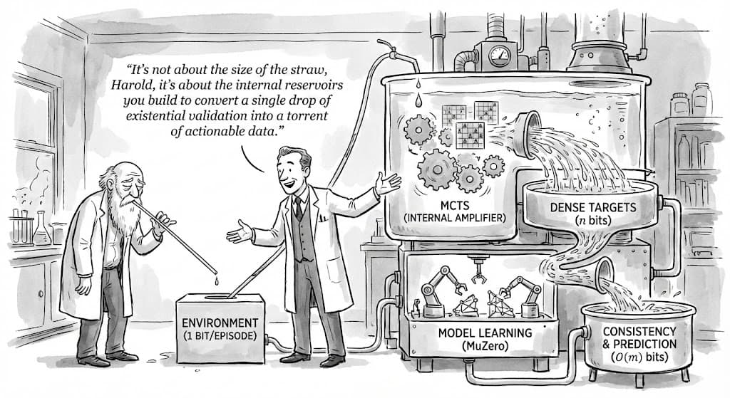
The relevant question for reasoning LLMs hence becomes: what’s the equivalent of MCTS for language? How do you build an internal amplifier that turns 1 bit from a solution checker into $O(T)$ bits of feedback about which reasoning steps were useful? Process rewards are one answer (at what cost though? Getting labels from humans? Using LLMs as judges? No way RL finds jailbreaks for high rewards, right? Right…?). Search over reasoning traces is another (learn to explore until you find correct paths, then distill). But both require solving their own hard problems.

---

Let’s get back to outcome-land though, there’s another point to be made here. Now that we have formalized the notion of 1 bit/episode in outcome-based RL, we are left with the other side of the original statement. Let’s make the missing link precise: why does a supervision channel that carries ~1 bit/episode naturally call for low-rank (LoRA-style) parameterization?

Chapter 2: Optimization

I’ll give (A) a structural/spectral argument that the task-relevant policy-gradient signal is intrinsically low-rank; (B) a complementary information/MDL capacity argument showing a small-rank adapter has enough coding capacity to absorb all the information the environment can deliver, whereas full FT unlocks far more degrees of freedom than the data can support; and (C) a compact theorem/proof packet.

1) Structure: terminal-reward PG produces low-dimensional signal at decision steps

For an affine layer $W_\ell\in\mathbb{R}^{d_{\text{out}}\times d_{\text{in}}}$, the per-episode REINFORCE gradient has the outer-product form

$G_\ell = \sum_{t=1}^T (R-b_t) u_{\ell,t} x_{\ell,t}^\top,$

where $u_{\ell,t}=\nabla_{\text{preact}_\ell}\log\pi(a_t\mid s_t)$ and $b_t$ is any baseline measurable w.r.t. $\tau_{\neg t}$ (action-independent). Each summand is rank-1, hence $\operatorname{rank}(G_\ell)\le \min\{T,d_{\text{out}},d_{\text{in}}\}$ for that episode. What matters, however, is that only decision steps carry signal in expectation, and at the output head that signal lives in a tiny subspace—often 1-D—under the checker.

Output-alignment lemma. Let $\mathcal D$ be the set of decision steps, and $S_t(Y)\subseteq{1,\dots,V}$ the success set at step $t$ (singleton $\{y\}$ in the usual case). Write $p_t\in\Delta^{V-1}$ for the token distribution, $u_{L,t}=e_{A_t}-p_t\in\mathbb R^V$ for the output-score gradient, and $q_t:=\sum_{s\in S_t(Y)}p_t[s]$. Assume:

1. (Checker sufficiency) $R$ depends on $\tau$ only through $Z_{\mathcal D}$ with $Z_t=\mathbf 1\{A_t\in S_t(Y)\}$ for $t\in\mathcal D$.

2. (Equivariance among non-success tokens) For any $k,k'\notin S_t(Y)$, $\mathcal L(R\mid\tau_{\neg t},A_t{=}k)=\mathcal L(R\mid\tau_{\neg t},A_t{=}k')$.

3. (Optional: symmetry among success tokens) For any $s,s'\in S_t(Y)$, $\mathcal L(R\mid\tau_{\neg t},A_t{=}s)=\mathcal L(R\mid\tau_{\neg t},A_t{=}s')$.

Then for every step $t$,

$\mathbb E \big[(R-b_t) u_{L,t}\bigm|\tau_{\neg t}\big] =\sum_{k=1}^V p_t[k] \left(\mathbb E[R\mid\tau_{\neg t},A_t{=}k]-\mathbb E[R\mid\tau_{\neg t}]\right)e_k.$

Consequently, if $t\notin\mathcal D$ the RHS is $0$ (no signal in expectation). If $t\in\mathcal D$, define $\mu_1(t):=\mathbb E[R\mid \tau_{\neg t},A_t\in S_t(Y)]$, $\mu_0(t):=\mathbb E[R\mid \tau_{\neg t},A_t\notin S_t(Y)]$; with Assumptions 2–3,

$\boxed{\mathbb E\big[(R-b_t) u_{L,t}\bigm|\tau_{\neg t}\big]=\big(\mu_1(t)-\mu_0(t)\big)\Big((p_t \circ \mathbf 1_{S_t})-q_t p_t\Big),}$

which lies in $\operatorname{span}\{e_s-p_t:\ s\in S_t(Y)\}$ (dimension $\le |S_t(Y)|$). In the singleton case $S_t(Y)=\{y\}$,

$\boxed{\mathbb E \big[(R-b_t) u_{L,t}\bigm|\tau_{\neg t}\big]=\big(\mu_1(t)-\mu_0(t)\big) p_t[y] (e_y-p_t),}$

i.e., a one-dimensional direction at the output.

Matrix view (output layer).

Let $W_{\text{out}}\in\mathbb R^{V\times d_{\text{model}}}$ and $h_t$ be the hidden state. The per-episode output gradient is

$G_{\text{out}}=\sum_{t=1}^T (R-b_t),u_{L,t},h_t^\top.$

By (3)–(4), only $t\in\mathcal D$ contribute in expectation; each such term is an outer product whose left factor lies in a subspace of dimension $\le |S_t(Y)|$ (singleton $\Rightarrow$ 1-D). Summing over $K:=|\mathcal D|$ decision steps yields, per episode, a sum of at most $\sum_{t\in\mathcal D}|S_t(Y)|$ rank-1 matrices. Averaging across a minibatch preserves the signal subspace (union of these few left-factor directions), though the exact matrix rank after averaging need not stay bounded by $\sum_{t}|S_t|$.

Takeaway. In checker-style, terminal-reward training, the signal-bearing part of each episode’s update at the output layer is confined to a tiny token-space subspace (1-D when $|S_t|=1$), and enters weights as a sum of very few outer products. This is precisely the structure LoRA is designed to capture.

2) Capacity: 1-bit/episode ⇒ small LoRA suffices at the information scale

Let the environment deliver $B$ bits over training (binary terminal rewards $\Rightarrow B\le n$ after $n$ episodes). A rank-$r$ LoRA update $\Delta W=AB$ has $P=r(d_{\text{out}}+d_{\text{in}})$ trainable reals; with $q$ effective bits/parameter, its description length budget is $\approx Pq$ bits (handwavy, but serves as an intuition). Thus a sufficiency heuristic is $Pq\gtrsim B$: the adapter can encode all the information the channel can supply, while full FT exposes $d_{\text{out}}d_{\text{in}}\gg r(d_{\text{out}}+d_{\text{in}})$ degrees of freedom—statistically under-regularized for such weak supervision. This aligns with MDL/PAC-Bayes-via-compression intuitions (generalization tracks description length, not raw parameter count) and with the intrinsic-dimension view that downstream changes often live in small subspaces.

3) Formal statements

Proposition 1 (Decision-local, low-dimensional RHS at the output).

Under checker sufficiency and equivariance, for any decision step $t$,

$\mathbb E\big[(R-b_t) u_{L,t}\bigm|\tau_{\neg t}\big]\in \operatorname{span}\{e_s-p_t:\ s\in S_t(Y)\},$

and it is $0$ for $t\notin\mathcal D$. In the singleton case $S_t(Y)={y}$, the span is 1-D. Consequently, the per-episode output-layer gradient is a sum over at most $K$ decision steps of outer products whose left factors lie in a subspace of dimension $\le \sum_{t\in\mathcal D}|S_t(Y)|$ (singleton $\Rightarrow \le K)$.

Proposition 2 (Rank preservation under left/right preconditioning).

If the parameter update is $\Delta W_\ell=L_\ell,G_\ell,R_\ell$ for some (possibly data-dependent but action-independent) matrices $L_\ell,R_\ell$, then $\operatorname{rank}(\Delta W_\ell)\le \operatorname{rank}(G_\ell)$.

Theorem (LoRA sufficiency via decision-local low rank + rank-preserving updates).

Fix a layer $W$ in the checker-style, terminal-reward setting. Assume:

1. (Decision locality) There are $K$ decision steps $\mathcal D$; at each, $S_t(Y)$ has size $\le s_t$ (singleton $\Rightarrow s_t{=}1$).

2. (Output alignment) Proposition 1 holds.

3. (Rank-preserving update) $\Delta W=L\bar G R$ for some left/right preconditioner (SGD: $L=R=I$; K-FAC: $L=\Sigma_u^{+},R=\Sigma_x^{+}$).

Then $\Delta W$ is $\varepsilon'$-close to rank $r$ with $\varepsilon'$ controlled by $\varepsilon$ and the operator norms of $L,R$. Therefore a rank-$r$ LoRA matches $\Delta W$ up to $\varepsilon'$.

​​Across depth, the information-carrying part of the gradient stays low-dimensional: with binary, terminal, checker-style rewards, the output-space error lives in a ~1-D subspace.

Backprop is linear in the output error: the layer-$\ell$ backprop signal satisfies

$(\delta_\ell = J_{\ell\to \mathrm{out}}^\top, g_{\mathrm{out}}),$

where $g_{\mathrm{out}}$ is the output-space error (here proportional to the PG term) and $J_{\ell\to \mathrm{out}}$ is the Jacobian of the forward map from layer $\ell$ to the output. Linear maps cannot increase the dimension of a subspace, so the image of a $k$-dimensional output subspace is $\le k$-dimensional at every earlier layer, so the expected $Y$-dependent gradient at any layer remains confined to a small union of directions.

---

What we have derived so far is that Outcome-based RL is a bandwidth-starved regime whose expected gradient lives in an extremely small subspace. This is great! Most implementations in the open still rely on ORMs, so you should really use LoRAs (and in particular, very low-rank adapters). But surely the Big Labs™ do some different kinds of shenanigans, right? Let’s try speculating (but not too much) very simple methods to increase bandwidth.

Chapter 3: Speculation

The claim I will try to make (albeit less rigorously, just at an intuitive level) is that rubric/PRM/RM-based RL widen the straw along both axes—more bits and more independent directions—so the expected gradient’s subspace expands accordingly. Low-rank adapters remain a good inductive bias, but the rank you will need scales with the number of independent supervision directions actually revealed, the number of decision steps carrying signal, and (practically) how many trajectories you average over. Let’s continue.

1) How supervision type shapes directions

Think in two orthogonal axes:

• Entropy (bits/episode): how many bits the feedback can transmit.

• Directional dimensionality (directions/episode): how many distinct logit-space directions the feedback distinguishes (i.e., how many ways it “pulls apart” wrong answers relative to each other).

The second axis is what breaks the equivariance assumption (“all wrong tokens are equivalent,” or better, credit assignment is token-independent). Once wrong answers are not treated symmetrically, the output-side signal no longer collapses to a single direction like $e_y - p$, but rather, it fans out across multiple basis vectors. A quick taxonomy

Directional rule of thumb (output layer): Let $D$ be the number of decision steps that carry signal and $K$ the number of independent feedback dimensions exposed (criteria, heads, or distinct action-dependences). Then the left-factor subspace of the expected output gradient is typically of dimension

$S_{\text{out}} \lesssim K \times D,$

2) How “asymmetric wrongs” break equivariance

Equivariance (“any wrong token behaves the same for reward”) implies the output-space expectation $\mathbb E[(R{-}b)u_{L,t}|\tau_{\neg t}]$ lies in $\mathrm{span}\{e_y - p_t\}$ at a decision step $t$. Rubrics/PRMs/RMs break this by assigning different expected reward deltas to different wrong tokens (or spans):

• Rubrics: Each criterion “lights up” distinct failure modes (e.g., correctness, reasoning, format). Revealing the vector $R^{(1:K)}$ turns a single scalar tug into a sum of $K$ tugs along different token subsets, expanding the left-factor span to $\le K$ directions at that step.

• PRMs: Token-/span-level signals distinguish where and how the trajectory deviated. The left-factor at time $t$ becomes a mixture of directions tied to those spans; summing across many steps yields $S_{\text{out}}$ scaling with the number of rewarded/penalized locations.

• RMs (single scalar): Even with a single scalar, the mapping from logits to score can be non-symmetric in the wrong tokens. If the reward is higher when you choose “almost-right” tokens (e.g., numerically near, semantically close), then the expected direction becomes a weighted combination of multiple $e_k - p$ vectors instead of just $e_y - p$.

Closing thoughts

I keep coming back to the decomposition

$I(Y;\mathcal H_n)=\sum_i I(Y;\tau_i\mid \mathcal H_{i-1})+\sum_i I(Y;R_i\mid \tau_i,\mathcal H_{i-1}),$

because it reframes a lot of recent RL-for-LLM work as choices about where to spend bits.

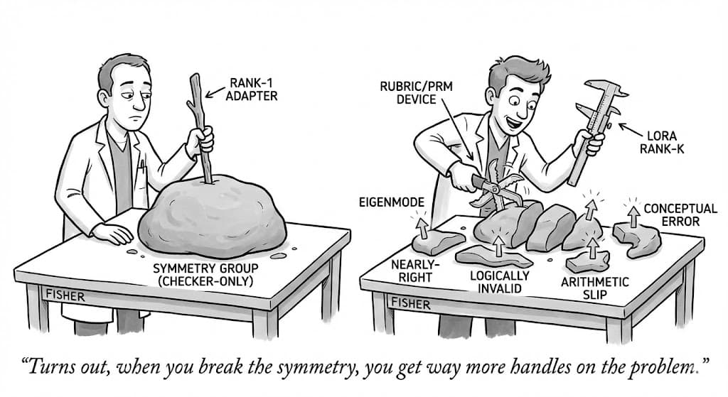
The part of my story that I hope people will have really metabolized by now is the symmetry claim. Binary checkers impose a group action on the output space. All wrong tokens become members of a single orbit: the reward is invariant to permutations among them. The policy gradient is therefore the gradient of a class function—constant on the “wrong” orbit and distinct on the singleton “right” orbit. That symmetry collapses the expected update into essentially one output-space direction, the “push mass from the wrong orbit to the right token” direction. Once you see it that way, a lot of the geometry in Chapter 2 falls out for free: you’re training on a function with a giant isotropy group, so the Fisher/Hessian has one salient eigenmode aligned with $e_y - p$ and a big flat subspace orthogonal to it. Low rank-ness becomes the right inductive bias because the loss landscape simply doesn’t expose more curvatures.

Breaking that symmetry is the core act of widening the supervision channel, and it’s more subtle than “add bits.” Rubrics, PRMs, and learned critics are symmetry-breaking devices. They split the wrong orbit into subclasses—nearly-right versus far-off; logically invalid versus stylistically off; arithmetic slip versus conceptual error. Each split adds an eigenmode to the curvature: more directions along which the loss can “pull apart” the logits. I think that if you looked at the empirical Fisher before and after adding a rubric head, you’d see previously degenerate mass reallocated into a handful of new eigenvectors corresponding to those failure modes. LoRA’s role then becomes almost spectral: pick a rank commensurate with the number of irreducible components you’ve activated by supervision. Supervision richness and representational rank should co-evolve. In the checker-only regime the symmetry group is huge; a rank-1 or rank-2 adapter is likely well aligned with the only active mode. As you break the group into $K$ subclasses with a rubric, the Fisher sprouts $K$ salient directions; keeping LoRA rank artificially tiny now becomes information-throttling rather than regularization.

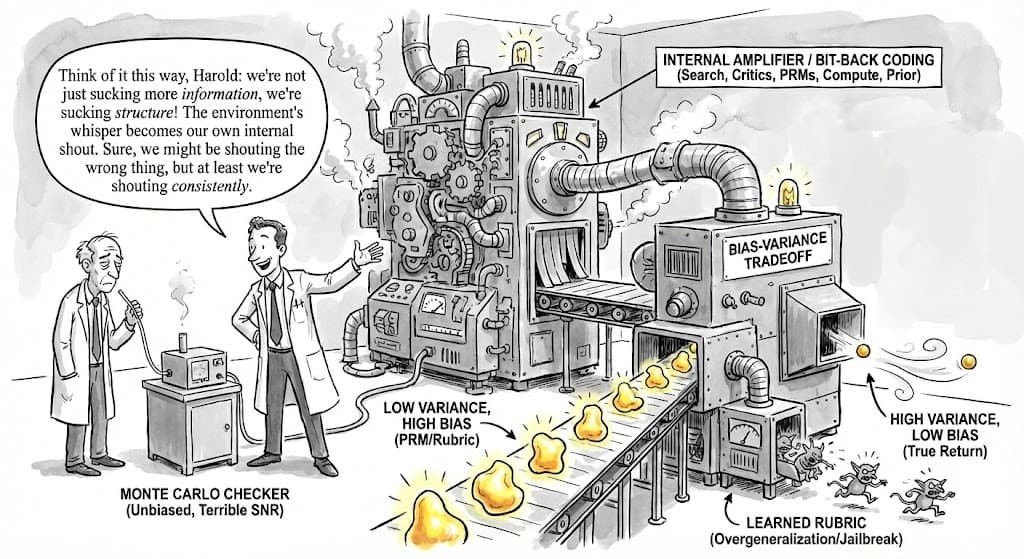
There is also a cleaner way to talk about the value of internal amplification that sidesteps the “but the environment still emits 1 bit” objection. The object we care about is the mutual information between our update and the gradient direction for return, not just $I(Y; R)$. In the binary-checker setting, the optimal direction is still $e_y - p$ at the output, but we typically don’t know where the decision steps are or which wrongs are “closer.” Search, critics, and PRMs increase this mutual information by injecting structure from the prior: compute and auxiliary models make the update less noisy around the right direction even though the raw environmental channel hasn’t changed. The early AlphaGo papers read like variance reduction tricks in this lens: MCTS computes a high-SNR surrogate target for many states; policy learning becomes matching those targets. You can view this as a form of bit-back coding: the 1 environmental bit seeds a lot of internally generated bits that are compressible because they are computed from a strong prior and many correlated rollouts. The environment didn’t speak more, but you used your prior to say a lot more to yourself.

This reframing clarifies the bias–variance trade when you replace verifiable outcomes with fuzzy rubrics. Monte Carlo policy gradients with a checker are unbiased for the true return gradient but have terrible SNR when success is rare; PRMs and rubrics supply dense signals with vastly lower variance but introduce bias because they’re not the true return. The right measure isn’t the MI with $Y$ (which a PRM can’t fundamentally increase by DPI if it sees the same $\tau$) but rather the risk for estimating $g*$: $MSE = bias^2 + variance$. There is a regime where adding a biased PRM reduces MSE because variance collapses faster than bias hurts, especially on long chains where MC success probability is exponentially small. There is another regime—distribution shift, misspecified preferences, jailbreaks—where bias dominates and you optimize the wrong thing spectacularly well. This is just the classic overestimation pathology in value learning wearing new clothes: a learned rubric is a value function over language; it will overgeneralize on states it hasn’t seen, and policy optimization will chase those blind spots. The practical antidotes from deep RL carry over: conservative objectives, pessimism under uncertainty, doubly robust estimators that mix outcome-based Monte Carlo with PRM predictions, and targeted data augmentation toward high-advantage, high-uncertainty regions. As a safetyist, maybe preference learning should be framed as a pessimistic risk minimization problem with uncertainty calibration, not as a pure regression to scalar rewards.

Exploration is the other half of the story we rarely import from Deep RL into LLMs. In language, we have a perverse inverse: the model is too confident in familiar patterns, so exploration looks like diversifying intermediate reasoning states rather than final answers. Given how intrinsic this is to pretraining, I find this to be one of the hardest problems, and likely the one whose solution would lead to the biggest gains.

Finally, it’s worth saying out loud that “internal bits” and “external bits” are different currencies. The environment bit is ground truth; every other bit we produce is a function of our prior and compute budget. Performance improves when internal bits line up with the true gradient. Generalization improves when external bits constrain us away from degenerate solutions that internal computation can hallucinate. An overlooked practical implication follows for rank and optimizer design. With only environment bits, the expected gradient lives in a tiny subspace; low-rank adapters with light or no preconditioning (SGD!) are both natural and robust. As you add internal bits via search, critics, and rubrics, the signal subspace grows. At that point, low rank is still helpful as a denoiser, but you should let the rank track the empirical spectrum, and you should switch to rank-preserving preconditioners (Muon?) that faithfully propagate those additional modes backward through depth. Put simply: match rank to the supervision algebra you actually exposed.

There’s a simple, operational way to tie all of this together. Keep a running “bit ledger” and a “direction ledger.” The bit ledger counts external bits you’ve bought: binary outcomes, human preferences, rubric criteria, tool verdicts. The direction ledger tracks how many independent logit-space directions those bits have actually activated, as measured by the spectrum of the empirical Fisher over tasks you care about. Match LoRA rank to the direction ledger, not the parameter count. Spend external bits where the direction ledger stalls, and spend compute where it already grows, by building the internal reservoirs that convert your one-bit world into a rich, structured gradient field you can actually follow.